Computer Science Fundamentals: Data Structures - Part 1
Continuing with our series on computer science fundamentals, lets take a look at some different data structures and when you would choose to use one or the other.
The name “data structure” initially sounds really intimidating but it really just means any object that contains data in a specified way. Data structures are used to collect different data points. If you wanted to constantly refer to the letters of the alphabet, it would be a real pain to type out each letter every time. It would be much easier to store each letter into one collection and refer to the collection over and over again rather than the individual letters. Let’s look at some of the different data structures available to us.
Arrays
An array is one of the most basic and fundamental data structures in any computer language. An array is a collection of objects that is indexable. This means that the array knows how many items are in its collection and it can almost instantly access a specified slot. Let’s imagine that I have an array called “alphabet” which stores each individual letter of the alphabet in a seperate slot. If I wanted to access the third item in an array called “alphabet” in Ruby you can call its index with the bracket notation
alphabet[2]
I know what you’re thinking. I made a mistake and should have written 3 rather than 2. It turns out that an array starts counting from zero so if I wanted the third element in the alphabet array, the above notation is correct.
Arrays have a couple of downsides. The first, is that they have a fixed size. When you create a new array, depending on the language, you either have to specify the size ahead of time or your language will specify a size for you. In C, you must specify the size of the array when it is created and that can’t be changed. In Ruby, a new array is initially created with 3 spaces. If you use those three, a new array will be dynamically created for you with 2o spaces and then the size roughly doubles from there. Every time you create a new, larger array and transfer over the contents you take a memory hit. In Ruby, if you’re creating a new large array and there isn’t enough memory you may trigger a garbage collection activity.
The second downside of an array is that adding new elements to an array can be a very expensive operation from a memory perspective. If you want to create a new item at the beginnng of an array, you have to shift every element down one slot. If you have an array with a million items, you might be sitting at your computer for awhile.
Linked Lists
Linked lists were created to solve some of the problems that arrays encounter. Instead of having a simple collection of objects, you have a series of linked nodes. Each node has two pieces of information associated with it. The first is the actual data you are storing, which would be the letter of the alphabet in the previous example. The second is a pointer to a memory location of the next node in the list. That’s it. There is no part of the Linked list that knows about the entire collection. Usually you have a object that points to the beginning of the linked list called the HEAD. You then follow each part of the linked list jumping from node to node until the memory pointer is set to null, or nothing. This is called the TAIL and it is how your computer knows it has reached the end of the list.
The linked list has several advantages over an array. The first is the inserting or deleting an object from the list is relatively painless from a memory perspective. If you need to insert an item at the beginning of a list you would create a new node that points to the original HEAD of the list and then update the HEAD pointer to point to your new node. Let’s say you have a list of items that you are keeping in alphabetical order. Each element in a parentheses represents a node with data and the pointer to the next node.
("apple", pointer to "ball") -> ("ball", pointer to "dog") -> ("dog", null)
Let’s say we wanted to insert “cat” between “ball” and “dog” in order to keep everything alphabetical. First, we would create a new node with the data set to “cat” and the pointer pointing to “dog”
("cat", pointer to "dog") -> ("dog", null)
We would then update the pointer for “ball” to point to the “cat” node rather than the “dog” node. The final order would look like this:
(“apple”, pointer to “ball”) -> (“ball”, pointer to “cat”) -> (“cat”, pointer to “dog”) -> (“dog”, null)
Note that the order that we performed the operation is important. If we had updated the “ball” node pointer to point to “cat” first, we would have lost any reference to “dog” and we would not have been able to find it in memory.
There are also disadvantages to using linked lists. The first is that finding an element could be quite painful with a Big O of N. If you’re not familiar with that terminology, check out my earlier Computer Science Fundamentals post on Searching and Sorting. If you wanted to find a specific element and check whether that is in the linked list, you would need to start at the beginning of the list and continue through each node, checking whether there is a match.
Additionally, the linked list has no idea how long the chain is or what’s contained within it so you can’t simply access the third element in the linked list by calling [2] on the list. Finally, a flaw that both arrays and linked lists have is that there is no concept of grouping. If I wanted to store all words that start with the letter “a” for quick retrieval, both arrays and linked lists would fail. To overcome some of these issues, we can use Hashes.
Hashes
Hashes are another fundamental data structure that combines elements of the two previous structures we’ve learned about in order to generate a new structure that solves some of the issues we spoke about previously.
The most important distinction with hashes its its lookup functionality. You can lookup a single object or a group of objects by a key that you set. You will sometimes hear hashes referred to as a set of key-value pairs. How the hash accomplishes this is actually pretty interesting.
When you create a hash and set a key, that key is run through a hashing algorithm. Books have been written about the different kind of hashing algorithms but what they all share is that they will reliably produce the same result each time. For instance, if the key of “apple” is run through a hashing algorithm and the algorithm produces the number “1”, that algorithm will always produce a value of 1 when given the key of apple.
Internally, hashes use arrays and linked lists in order to construct the data structure. The key is run through a hashing algorithm, which produces a certain value. That value will map to a specific slot within an array and the value will be pushed into that slot. Imagine that the keys we’re dealing with are only integers and the hashing function is the modulo operator which finds the remainder of a number. We can set up an array with a size of five and process every input with a modulus of 5. The operator will always produce a number from 0 to 4. For example, if the key we’re trying to assign is 107, we will process that through our hashing algorithm:
107 % 5 #=> 2
The key of 107 will always map to the third slot in the array, which will be filled by whichever value you decide. Now if you want to access the value associated with the key of 107, you can reliably run it through the hashing algorithm knowing that it will find the same value almost instantaneously.
In order to help visualize this process I borrowed an image from Wikipedia.
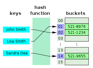
Here, the keys are names of people and the values are their phone numbers. The keys are run through a hashing function which is unknown but it reliably maps the key to the same bucket each time.
There are a couple of obvious problems though. The first is the collision problem. Let’s return to our previous example. We’ve now run 107 through our hashing algorithm which is just the modulus operator and we placed the value associated in the third bucket. What happens if we run the hashing algorithm with a key of 212?
212 % 5 #=> 2
It maps to the same bucket! We have a collision here and there are a couple ways that hashes solve this. The most common way is called separate chaining. In separate chaining, if we have a collision, then the location in the array bucket above is turned into a linked list. So if we imagine the 107 mapped to “Matz” and 212 mapped to “Ruby”, the third slot in the array will look like a regular linked list.
("Matz", pointer to "Ruby") -> ("Ruby", null)
However, if we were to let the linked list grow too big, we would run into the same performance problems that we’ve identified previously. To solve this, most hashing tables will limit the length of the linked list in each array. What happens when those limits are reached? That brings us to another problem associated with hashes. The hash will need to rebuild with a larger array bucket and then rerun every key through the hashing algorithm in order to replace the values. Obviously this becomes an intensive memory operation but hopefully it won’t happen too often.
Wrapping Up We learned about some of the most fundamental data structures in computer science. In Part 2 of this post we will explore heaps, trees, queues, stacks and graphs. Stay tuned!
As always, hit me up on Twitter if you have any questions @danielspecs and let me know if you have any feedback on the points above.